Bridging engineering, design, and business
— from idea to prototype to market
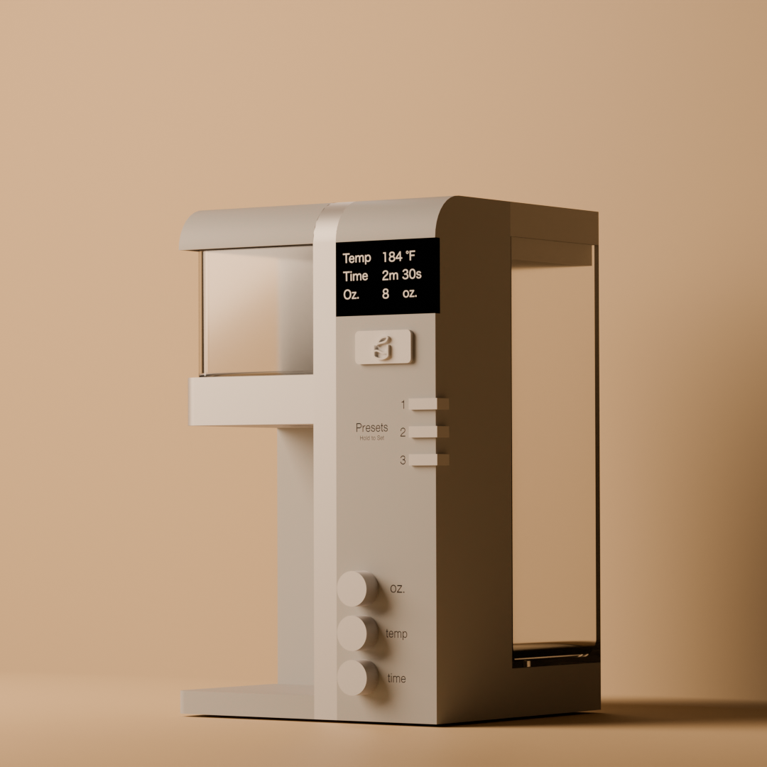
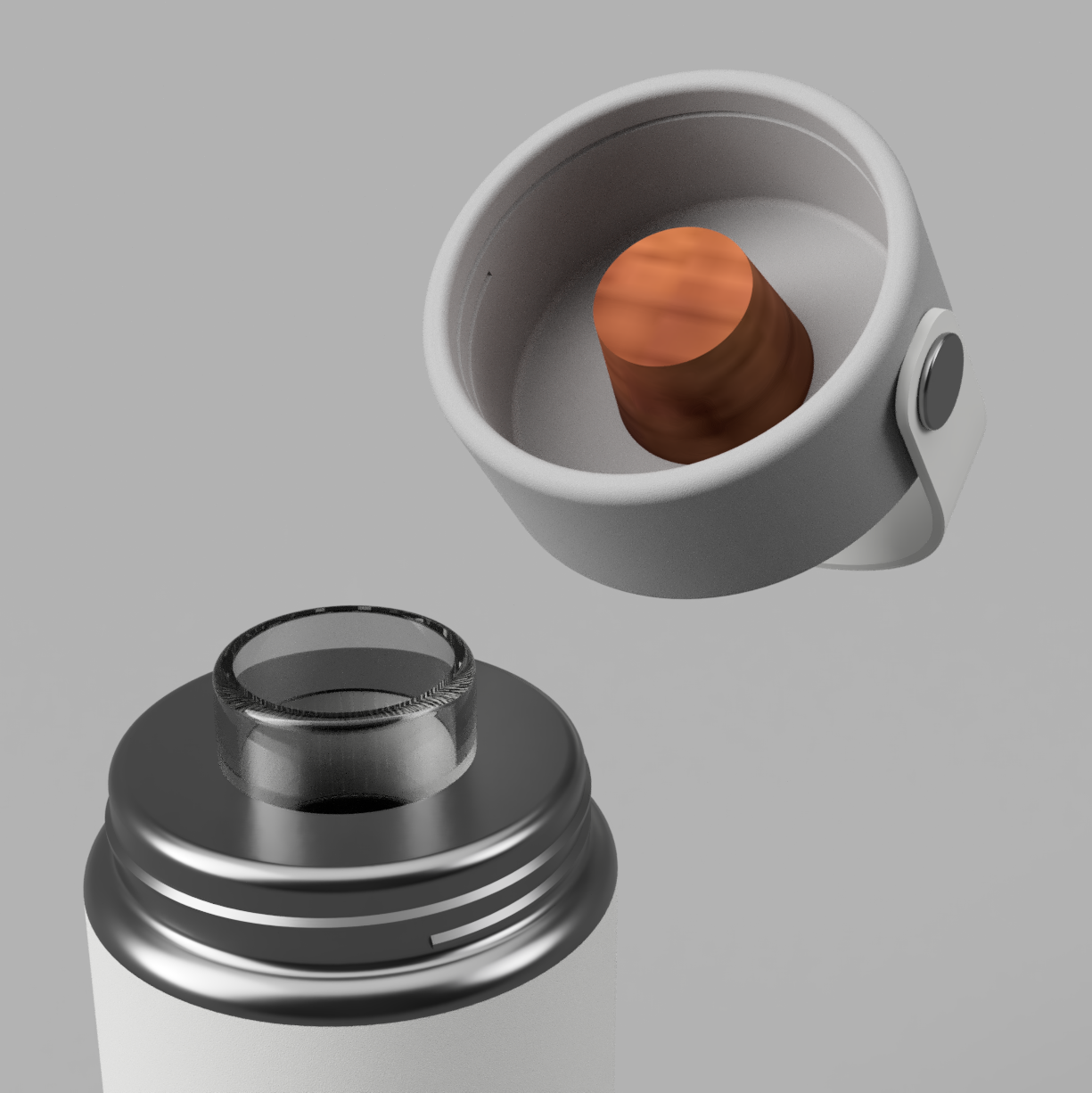
Concept-to-deployment product lifecycle
Iterative prototyping to in-house pilot builds
User research, customer research, and pilot testing to inform design decisions
Robotics, mechatronics, and computer vision design and development
Cross-functional teamwork and collaborative design processes
Market analysis, competitive analysis, and business strategy development